The core problem of machine learning boils down to learning a function with parameters such that given data, the model is able to give the desired output. This the model does by iteratively looking at multiple instances of labelled data and fixing its parameters, small steps at a time. We use this approach to train our first model and predict Boston Housing Prices and – Wallah – a new ML engineer is born. But is it really that straightforward? Turns out things get really intense, murky, and chaotically beautiful when we look at the problem from a statistical perspective.

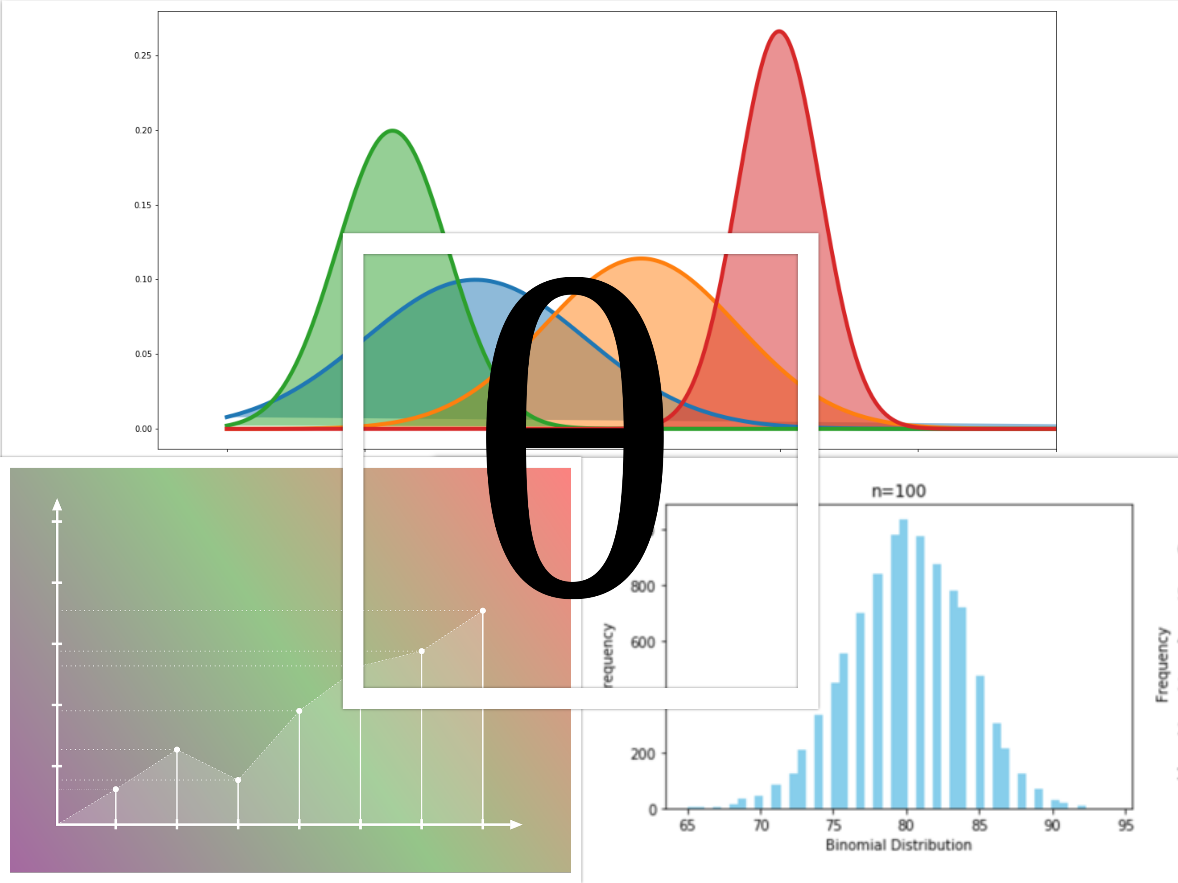
Let’s consider a Probabilistic Model of the problem: $y^{(i)} = \theta^T\textbf{X}^{(i)}+\epsilon$ Here, $y$ represents the output, $\theta$ the weights, $\textbf{X}$, and $\epsilon$ the error/noise associated with the output which we get as a part of the output. Now, some might be confused as to why the error/noise? To them – the thing is, we never are able to get clear output from model; if we did, our models will be capable of emulating exactly whatever process/ system we are trying to model and will have an accuracy of 100 percent which is almost never the case, and thus, the pesky noise. Like it or not, we get the noise; how to deal with it, that is the question.

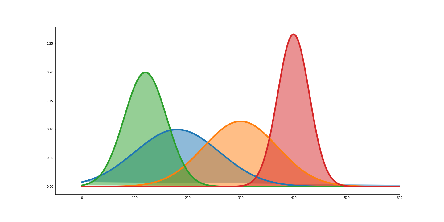
We consider the noise to follow a Gaussian/ Normal distribution and move ahead **. . . **

Why Gaussian you ask? Okay, let’s go over it:

A Gaussian Distribution makes sense because noise results from a large number of independent variables; the result of summing up a large number of different and independent factors allows us to apply the Cen­tral Limit Theorem which states that the sum of independent random variables is well approximated (under rather mild conditions) by a Gaussian random variable, with the approximation improving as more variables are summed in. I will not go further into this but if noise has piqued your interest, here is something to get you started.

Having put the curious case of noise to rest (somewhat), let’s go ahead and actually model the $\epsilon$ as Gaussian. The PDF of a Gaussian Distribution is given as : $p(x^{(i)};\mu,\sigma^2) = \frac{1}{\sqrt{2\pi}\sigma}\exp{\frac{-(x^{(i)}-\mu)^2}{2\sigma^2}}$ where parameters $\mu$ and $\sigma^2$ denote mean and variance respectively. Now, since, we need to model the noise, we will parameterize our model with $\epsilon$:
$p(\epsilon) = \frac{1}{\sqrt{2\pi}\sigma}\exp\frac{-(\epsilon^{(i)})^2}{2\sigma^2}$ From $(1)$ we can write $\epsilon$ as $y-\theta^T\textbf{X}^{(i)}$; using it in $(3)$, we get:
$p(y^{(i)}|\textbf{X}^{(i)};\theta) = \frac{1}{\sqrt{2\pi}\sigma}\exp\frac{-(y-\theta^T\textbf{X}^{(i)})^2}{2\sigma^2}$

Now that we have a probabilistic model in place where the function is parameterised by $\theta$ , and observed data at hand, we need to find out parameters that maximise the chance of seeing the observed data. For this, we need to pick out another tool from our tiny little bag of statistics: the Maximum Likelihood Estimator (MLE). This MLE function is parameterised by $\theta$ , so we can write: $L(\theta;\textbf{X},y) = p(y|\textbf{X};\theta)$ Note that the equation in $(4)$ is just for one data point. In order to extend it to the whole data set, we write the likelihood function as : $L(\theta) = \prod_{i=1}^{N} \frac{1}{\sqrt{2\pi}\sigma}exp-{\frac{(y-\theta^T\textbf{X}^{(i)})^2}{2\sigma^2}}$ Above is the likelihood function for $\theta$ which we need to maximise by the same old gradient descent, but here we are maximising, so add instead of subtract – differentiate the function and add to the current value – thus making it gradient ascent. Let’s go ahead and do that.

What … why’d you falter? Oh, yeah the function $L(\theta)$ is not quiet easy to differentiate. Okay, we see a product and an exponential function; what can we do? Aha!! square the function – nah, that makes it nastier. How about a $log_e$ ? It takes care of the products by turning them into sums and removes the exponential function making the overall expression much more amenable. This also preserves the overall increasing nature of the initial function as $log$ is also an increasing function. Hence,we can maximise any strictly increasing function of $L(\theta)$ instead of $L(\theta)$ itself.

Skipping the intermediate, straightforward, parts: $l(\theta) = logL(\theta) = N.log\frac{1}{\sqrt{2\pi}\sigma} - \frac{1}{2\sigma^2}\sum_{i=1}^{N}(y^{(i)}-\theta^T\textbf{x}^{(i)})^2$ Upon differentiating above equation with respect to $\theta$, we are left with: $\frac{1}{\sigma^2}\sum_{i=1}^{N}(y^{(i)}-\theta^{(T)}\textbf{x}^{(i)})\textbf{x}^{(i)}$ For one data point, it will be: $\frac{1}{\sigma^2}(y^{(i)}-\theta^{(T)}\textbf{x}^{(i)})\textbf{x}^{(i)}$ which resembles the update value for gradient descent. The final update rule for parameter $\theta^{(i)}$ becomes: $\theta^{(i)} = \theta^{(i)}+\alpha(y^{(i)}-\theta^{(T)}\textbf{x}^{(i)})\textbf{x}^{(i)}$

$\sigma^2$ does not play a role in finding the parameters, so we neglect them. I’m yet completely explore as to why exactly we ignore the variance or set it to 1, but it might be something along the lines of maximizing likelihood means minimizing variance for optimal conditions.[Will Update on this later]

So, we end up with an expression similar to that of the update rule for minimising the error of the model. Well that’s satisfying.

Bear with me a little more and let’s look at the MLE for Logistic Regression.

Logistic Regression or the Bernoulli Linear Models (Bernoulli because it takes values between 0 and 1 –why? you’ll know from the range once we define the function) is a model that enables binary classification. We use a function that takes values that lies in ${[0,1]}$. The logistic function is represented as : $h(x) = \frac{1}{1+e^{-\theta^Tx}}$ . Using the assumptions about the probability distribution to be: $p(y=1|x;\theta) = h_\theta(x)\\ p(y=0|x;\theta) = 1 - h_\theta(x)$ as our model is binary and takes two values only.

A general equation for the value of a data can be written as: $p(y|x;\theta) = (h_\theta(x))^y(1-h_\theta(x))^{1-y}$ Using above p.d.f., the likelihood function for $\theta$ is given by : $L(\theta) = \prod_{i=1}^{N}(h_{\theta}(x^{(i)}))^{y^{(i)}}(1-h_{\theta}(x^{(i)})^{(1-y^{(i)})})$ Using similar approach as above (skipping intermediate steps), we consider the log-likelihood: $l(\theta) = \sum_{i=1}^{N}y^{(i)}log(h_{\theta}(x^{(i)}))(1-y^{(i)})log(1-h_{\theta}(x^{(i)}))$ whose derivative with respect to $\theta$ is: $(y-h_{\theta}(x^{(i)}))x^{(i)}$ , and if we use gradient ascent to maximise the likelihood of $\theta$ as before, we get: $\theta_j = \theta_j+\alpha(y_{(i)}-h_{\theta}(x^{(i)}))(x^{(i)})$

whose structure is very similar to what we obtained for the linear regression, also $h_{\theta}(x^{(i)})$ does not represent $\theta^Tx^{(i)}$ here.

**Why though? Is it just a mere coincidence or something connects these linear models? **

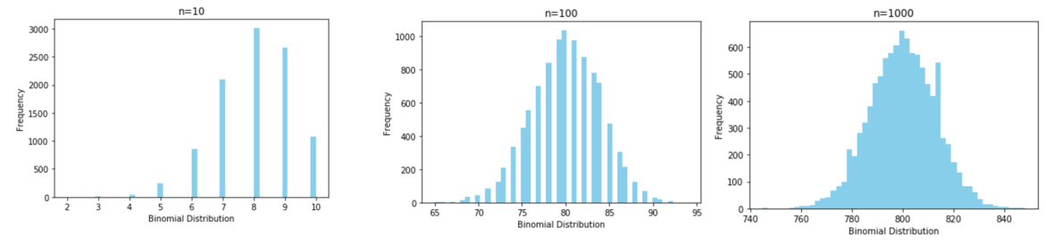
Answer to this is: Exponential Family of Distribution. It turns out to be the case that most of our common distributions like Bernoulli, Binomial, Normal and others. A couple that do not belong to this class include uniform and t distribution. Why the discrimination though? Simply because for the Uniform distribution, when the bounds are not fixed, the support of the distribution depends on the parameter and does not remain fixed across all parameter settings; the t-distribution doesn’t have the form that follows the exponential family. Check out the examples section here for more on this.

Exponential Family of distributions are defined by: $p(y;\eta) = b(y)(\eta^TT(y)-a(\eta))$ where $\eta$ represents the natural parameter, $T(y)$ represents the sufficient statistics, and $a(\eta)$ represents the log partition function. Another form of the Exponential family as described in the Machine Learning book by Kevin Murphy is: $p(x|\theta) = \frac{1}{Z(\theta)}h(x)exp[\theta^T\phi(x)]$ where $Z(\theta) = \int_{\chi^m} h(\textbf{x})exp[\theta^T\phi(\textbf{x})]dx$ such that $A(\theta) = logZ(\theta)$ ​ . So, $Z(\theta)$ can be written as
$exp(A(\theta))$ and hence the equation in $(19)$ becomes, $h(x)exp[\theta^T\phi(x)-A(\theta)]$

In the equation $(18)$ above, $\eta$ stands for the canonical or the natural parameter, $T(y)$ (a value which contains all the information to compute any estimate of the parameter: Wikipedia ) denotes the sufficient statistics of the distribution, and $a(\eta)$ denotes the log partition function. I decided not to delve deep into these individual building blocks of the equation as each of them make up their own area of study. But a very cool property of the log partition function, which I just want to put forth is that its derivatives give the cumulants of the sufficient statistics. The first and second cumulants of a distribution are the mean and variance. Doesn’t it sound familiar to the moments of a distribution where we could take derivatives of a certain function which would give us the moments of that distribution at $\textbf{X}$, $\textbf{X}^2$,$\textbf{X}^3$ and so on. To parallel that, there also exists a cumulant generating function that is unique to every distribution. To see if this actually work, let us set a couple of known probability distributions and see if the derivatives to their log partition function really does give rise to cumulants.

Starting with the Bernoulli distribution, we can write it as : $p(y;\phi) = \phi^y(1-\phi)^{(1-y)}\\$ Using $exp$ and $log$ to restructure the formula: $= exp(y\hspace{5pt}log(\phi)+(1-y)\hspace{5pt}log(1-\phi))$

$$= exp((log\frac{\phi}{1-\phi})y+log(1-\phi))$$

Above is the representation of Bernoulli distribution as an exponential family where $T(y) = y$, $a(\eta) = -log(1-\phi)$, $\eta = log\frac{\phi}{1-\phi}$, and $b(y) = 1$ according to the representation in $(18)$.

From, $\eta = \frac{\phi}{1-\phi} \implies \phi = \frac{1}{1+e^{-n}}$. So, $a(\eta) = log(1+e^{\eta}) \\ \frac{d[a(\eta)]}{d\eta} = \frac{e^{\eta}}{1+e^{\eta}}$

$$= \frac{1}{1+e^{-\eta}} = \mu$$

Upon double differentiating, we get, $\frac{d^2a}{d\eta^2} = \frac{d\mu}{d\eta} = \mu(1-\mu)$

Since we modelled the noise in our model as Gaussian, let’s see how it can represented in the form of an exponential family: $p(x|\mu,\sigma^2) = \frac{1}{\sqrt{2\pi}\sigma}exp\frac{-(x-\mu)^2}{2\sigma^2}$

$$= \frac{1}{\sqrt{2\pi}\sigma}exp\frac{-(x^2-2\mu x+\mu^2)}{2\sigma^2}$$ $$= \frac{1}{\sqrt{2\pi}}exp(-\frac{x^2}{2\sigma^2}+\frac{\mu x}{2\sigma^2}-\frac{\mu^2}{2\sigma^2}-log\sigma)$$

above, $\frac{1}{\sigma} = exp(-log\sigma)$ is used $= \frac{1}{\sqrt{2\pi}}exp(\frac{\mu x}{\sigma^2} - \frac{x^2}{2\sigma^2} - (\frac{\mu^2}{2\sigma^2}+log\sigma))$ where, $\eta = \begin{bmatrix} \frac{\mu}{\sigma^2} \\ -\frac{1}{2\sigma^2} \end{bmatrix};\hspace{5pt} T(y) = \begin{bmatrix} x\\ x^2 \end{bmatrix};\hspace{5pt} a(\eta) = \frac{\mu^2}{2\sigma^2}+log\sigma; \hspace{5pt} b(y) = \frac{1}{\sqrt{2\pi}}$ Here, we can differentiate either with respect to $\eta_1 = \frac{\mu}{\sigma^2}$ or $\eta_2=\frac{-1}{2\sigma^2}$ for we have a matrix. Before differentiating, $a(\eta)$ needs to converted in terms of $\eta_1$ and $\eta_2$ which is straightforward. Then upon differentiating, we get: $\frac{\part[a(\eta_1,\eta_2)]}{\part\eta_1} = \frac{\eta_1}{2\eta_2} = \mu$ Taking the second derivative yields, $\frac{\part^2a}{\part\eta_1^2} = \frac{-1}{2\eta_2} = \sigma^2$ So, as you see, the cumulant function gives the cumulants to the distribution. But this is not specific to these distributions. It is shown mathematically (check Kevin Murphy’s ML Book - Page 287 for proof) that $\frac{da}{d\theta} = \textbf{E}[T(y)];\hspace{5pt} \frac{d^2a}{d\theta^2} = \textbf{E}[T^2(y)]-\textbf{E}[T(y)]^2 = Var[T(y)]$ which can be extended to multivariate cases.

There is a lot of other interesting results like the Maximum Likelihood Estimator of Exponential family, convexity of the partition function among others about which you can read in the documents linked below if you wish to explore the area. Let’s move ahead.

Now that it’s visible that there exists a unifying force between the two models that we started with, let us now finally go ahead and derive them using the exponential family and a couple assumptions whose basis is rooted in the construction of the general equation of a linear model (check Section 9.3 Kevin Murphy’s ML Book). The assumptions about conditional distribution of $y$ given $x$ and about our model:

• y	x;$\theta$ ~ Exponential Family($\eta$) , i.e, $y$ follows an exponential family distribution with parameter $\eta$.

• Given data, our goal is to predict the expected value of $T(y)$ given data. T(y) = y (for most cases), so we would like our prediction to equal the expected value $\textbf{E}[y

  x] = h(x)$ . This is also justified for logistic regression as $h_{\theta}(x) = p(y=1

  x;\theta) = 0.p(0

  x;\theta)+1.p(1

  x;\theta) = \textbf{E}[y

  x;\theta]$

• Natural Parameter is related to the inputs as $\eta = \theta^Tx$. Prof. Andrew Ng’s notes from CS 229 clubs this one as a design choice for constructing GLMs but you can find where this comes from in Kevin Murphy’s ML Book [Section 9.3].

With everything set, let’s consider the Linear Regression model/ Ordinary Least Squares:

• We model $y

  x$ as Gaussian($\mu, \sigma^2$).

• $h(x) = E[y

  x;\theta]$. From assumption 2 above.

• $E[y	x;\theta] = \mu$

• $\mu = \eta$ . This comes from the fact that when deriving linear regression, the variance has no effect on the final output and parameters. So, if $\sigma^2 = 1$, the equality follows.
• $\eta = \theta^Tx$ . From third assumption.

Similarly, for logistic regression:

• $h(x) = E[y

  x;\theta]$

• $E[y	x;\theta] = \phi$

• $\phi = \frac{1}{1+e^{-\eta}}$ = $\frac{1}{1+e^{-\theta^Tx}}$

We see how both of these unique regression algorithms can be derived using the same set of assumptions based solely upon the type of distribution the outputs follow. The reason being these distributions belonging to a class of distributions called the Exponential Family of Distributions which caused likelihoods to be similar and the update rules to take the same form. This property is not limited to these distributions. Distributions like Poisson can be used to make models that are dependent on time, Multinomial distribution to classify emails as spam or not-spam (this turns out to be the Softmax regression), and other specialized linear models. There definitely exists a great deal about the Exponential Family and Generalised Linear Models that this post doesn’t cover and I do not know of and I’d want to explore it sometime, but it just feels great when the concepts are shown to have an abstract origin thereby allowing you appreciate them.

This post includes information gathered from my study of Prof. Andrew Ng’s CS 229 lecture notes -1, Kevin Murphy’s Machine Learning A Probabilistic Perspective, this lecture not from UC Berkeley, some Stack Overflow question, and definitely Wikipedia. Hence, the equations and terminologies used are derived/ used from these places and not of my own creation.

Source for images used: 1, 2, 3, 4